CISC 181 – 3002 Principles of Information Systems 13140
Steps to Perform:
| Step | Instructions |
| 1 | Start Access. Open the downloaded Access file named exploring_a01_grader_h1. |
| 2 | Open the Publishers table in Datasheet view. Add the following records to the Publishers table: PubID PubName PubAddress PubCity PubState PubZIP KN Knopf 299 Park Avenue New York NY 10171 BB Bantam Books 1540 Broadway New York NY 10036 PH Pearson/Prentice Hall 211 River Street Hoboken NJ 07030 SS Simon & Schuster 100 Front Street Riverside NJ 08075 Close the table. |
| 3 | Open the Books table and create a new record: AuthorCode: 15 Title: The Innocence Game ISBN: 0-307-96125-7 PubID: KN PublDate: 2013 Price: 24.95 StockAmt: 250 |
| 4 | Sort the records in the Books table by the PublDate field in descending order. Save and close the table. |
| 5 | Open the Maintain Authors form. In record 2 (for Keith Mulbery, AuthorID 12), add a new title to the subform: Title: Computer Wisdom III ISBN: 0-684-80417-5 PubID: PH PubDate: 2017 Price: 32 StockAmt: 42 |
| 6 | Use the Navigation bar to search for AuthorID 16, and then edit the subform so that the StockAmt is 6 instead of 496 for the book Follow the Stars Home. |
| 7 | Open the Publishers, Books, and Authors report and check that the report shows three books listing Keith Mulbery as author. View the layout of the report in Print Preview. Open the Publishers, Books, and Authors query. Sort the query by the publisher’s name in ascending order. |
| 8 | Use filter by selection to show only the books by the author whose first name is Steven. |
| 9 | Sort the query by Title in ascending order. Save and close the query. |
| 10 | Open the Books table. Use Filter by Form to create a filter that will identify all books published after 2010 with fewer than 100 items in stock. Apply the filter and preview the filtered table. Close the table and save the changes. |
| 11 | Close all database objects. Close the database and then exit Access. Submit the database as directed. |
| Step | Instructions |
| 1 | Start Access. Open the downloaded Access file named exploring_a02_grader_h1. |
| 2 | Create a new table in Design view using the name Donations. Add the primary key field as DonationID with the Number Data Type and a field size of Long Integer. Add the following field names to the table: DonorID, PlantID, DonationDate, and DonationAmount (in that order). |
| 3 | Change the Data Type for the DonorID and PlantID fields to Number. Change the Data Type for the DonationDate field to Date/Time, and then change the Data Type for the DonationAmount field to Currency. |
| 4 | View the table in Datasheet view, save the table, and then add the following records to the Donations table: DonationID DonorID PlantID DonationDate DonationAmount 1 24 15 3/17/2018 120 2 9 11 4/3/2018 50 3 14 9 4/19/2018 150 4 3 4 4/12/2018 60 5 18 7 4/19/2018 50 6 14 11 3/12/2018 125 |
| 5 | Sort the records in the Donations table by the DonationAmount field in descending order. Save and close the table. |
| 6 | Import the downloaded a02_grader_h1Plants.xlsx workbook as a new table in the current database. Using the wizard, specify that the first row contains column headings, set the PlantID field to be indexed with no duplicates, and set the PlantID field as the primary key. Import the table with the name Plants and do not save the import steps. |
| 7 | View the Plants table in Design view and change the field size for the PlantID field to Long Integer. Save the table. Click Yes in the dialog box indicating that some data may be lost. Close the table. |
| 8 | Begin establishing relationships in the database by adding the Donations, Donors, and Plants tables to the Relationships window. Close the Show Table dialog box. Create a one-to-many relationship between the DonorID field in the Donors table and the DonorID field in the Donations table, enforcing Referential Integrity. Select the option to cascade update the related fields. |
| 9 | Create a one-to-many relationship between the PlantID field in the Plants table and the PlantID field in the Donations table. Enforce Referential Integrity. Select the option to cascade update the related fields. Save and close the Relationships window. |
| 10 | Create a query using the Simple Query Wizard. From the Donations table, add the DonorID and DonationAmount fields (in that order). Ensure the query is a Detail query. Name the query Donations Over 100 and finish the wizard. |
| 11 | View the query in Design view, and then set the criteria for the DonationAmount field so that only donations greater than 100 are displayed. |
| 12 | Sort the query in ascending order by the DonationAmount field. Save the query. Run the query, and then close the query. |
| 13 | Create a new query in Design view. Add the Donations, Donors, and Plants tables to the query design window. Close the Show Table dialog box. Add the DonationDate field from the Donations table, the donor’s Lastname, Firstname, and Phone fields from the Donors table (in that order). |
| 14 | Add the DonationAmount field from the Donations table after the Phone field, and then add the PlantName field from the Plants table. |
| 15 | Sort the query in descending order by the date of the donation, and then by the last name of the donor in ascending order. Save the query with the name Plant Pickup List, and then run the query. Close the query. |
| 16 | Copy the Plant Pickup List query, and paste it using ENewsletter as the query name. |
| 17 | Open the ENewsletter query in Design view, and delete the DonationDate column. Add the ENewsletter field to the first column of the design grid and set it to sort in ascending order, so that the query sorts first by ENewsletter and then by LastName. Run, save, and close the query. |
| 18 | Close all database objects. Close the database and then exit Access. Submit the database as directed. |
Step
Instructions
1
Start Access. Open the downloaded Access file named exploring_a03_Grader_h1.
2
Create a query using Query Design. From the Customers table, include the fields CompanyName, ContactName, ContactTitle, and Phone (in that order). From the Orders table, include the fields OrderID, OrderDate, and ShippedDate (in that order). Run the query and then examine the records. Save the query as Shipping Efficiency.
3
Add a calculated field named DaysToShip to calculate the number of days taken to fill each order. (Hint: the expression will include the OrderDate and ShippedDate fields; the results will not contain negative numbers.) Run the query and then examine the results. Save the query.
4
Add criteria to limit the query results to include any order that took more than 30 days to ship.
5
Add the Quantity field from the Order Details table and the ProductName field from the Products table to the query (in that order). Sort the query by ascending CompanyName.
6
Add the caption Days to Ship to the DaysToShip field. Switch to Datasheet view to view the final results. Save and close the query.
7
Create a query using Query Design and add the Orders, Order Details, Products, and Customers tables. Add the fields OrderID and OrderDate (in that order) from the Orders table. Set both fields’ Total rows to Group By.
8
Add a calculated field in the third column. Name the field ExtendedAmount. This field should multiply the quantity ordered (from the Order details table) by the unit price for that item (from the Products table). Format the calculated field as Currency and change the caption to Total Dollars. Change the Total row for the ExtendedAmount field to Sum.
9
Add a calculated field in the fourth column. Name the field DiscountAmount. The field should multiply the number of items ordered, the price per item, and the discount field(in that order). This will calculate the total discount for each order. Format the calculated field as Currency, and add a caption of Discount Amt. Change the Total row to Sum. Run the query. Save the query as Order Summary. Return to Design view.
10
Add criteria to the OrderDate field so only orders made between 1/1/2016 and 12/31/2016 are displayed. Change the Total row to Where. This expression will display only orders that were created in 2016. Run the query and view the results. Save and close the query.
11
Create a copy of the Order Summary query named Order Financing. Switch to Design view of the new query and remove the DiscountAmount field.
12
Add a new field using the Expression Builder named SamplePayment. Insert the Pmt function with the following parameters:
• Use .05/12 for the rate argument (5% interest, paid monthly)
• Use the number 12 for the num_periods argument (12 months)
• Use the calculated field ExtendedAmount for the present_value
• Use 0 for both future_value and type
13
Change the Total row to Expression for the SamplePayment field. Change the Format for the SamplePayment field to Currency. Run the query and verify the second order has a sample payment of $125.84. Note: it will display as a negative number. Save and close the query.
14
Create a copy of the Order Summary query named Order Summary by Country. Replace the OrderID field with the Country field in Design view of the new query.
15
Run the query and then examine the summary records; there should be 5 countries listed. Switch to Design view and change the sort order so that the country with the highest ExtendedAmount is first and the country with the lowest ExtendedAmount is last. Run the query and verify the results. Save and close the query.
16
Close all database objects. Close the database and then exit Access. Submit the database as directed.
Step
Instructions
1
Start Excel. Download and open the file named e01_grader_h1.xlsx.
2
Merge and center the Travel Expense Report title in the range A1:E1.
3
In cell E5, enter a formula that calculates the number of days between the return date and the departure date.
4
In cell B12, enter a formula to calculate the amount budgeted for Mileage to/from Airport. The amount is based on the Mileage Rate to/from Airport and the Roundtrip Miles to Airport located in the Standard Inputs section.
5
In cell B13, enter a formula to calculate the amount budgeted for Airport Parking. Use the Airport Parking Daily Rate and calculate the number of total days traveling (use the # of Nights+1 in your formula) to include both the departure and return dates. For example, if a person departs on June 1 and returns on June 5, the total number of nights at a hotel is 4, but the total number of days the vehicle is parked at the airport is 5.
6
In cell B17, enter a formula to calculate the amount budgeted for Hotel Accommodations. This amount is based on the # of Nights, the Hotel Rate/Night, and the Hotel Tax Rate. In parentheses add the Hotel Tax Rate to 1 to equal 118% percent before multiplying.
7
In cell B18, enter a formula to calculate the amount budgeted for Meals. This amount is based on the Daily Meal Allowance and the total travel days (# of Nights+1).
8
In cell D12, enter a formula to calculate the difference between the Actual and Budget. Copy the formula to the range D13:D19. Delete the formula in cell D15. If the Actual expense is more than the Budget expense, the result is positive. If the Actual expense is less than the Budget expenses, the result is negative, indicating under budget.
9
In cell E12, enter a formula to calculate the % of Budget by dividing the Actual expense by the Budget expense to indicate the percent of the budgeted amount used in that category. Copy the formula to the range E13:E19. Delete the formula in cell E15.
10
Insert a new row 19. Type Other in cell A19. Bold the label. Delete the formula in cell E19.
11
Indent twice the labels in the ranges A12:A14, A16:A18, and A20.
12
Apply Accounting Number Format to the ranges B12:D12 and B21:D21.
13
Apply Comma Style to the range B13:D20.
14
Apply Percent Style with one decimal place the range E12:E20.
15
Ensure that the Comma style is applied to the range B20:D20. Use the Underline button to underline the range B20:D20. Do not use the border feature.
16
Apply the cell style Bad to cell D21 because the trip went over budget.
17
Select the range A10:E21 and apply Thick Outside Borders.
Note, depending upon the version of Office being used, the border may be named Thick Box Border.
18
Select the range A10:E10 and apply Blue-Gray, Text 2, Lighter 80% fill color. Apply Center alignment and apply Wrap Text.
19
Set a 1.5-inch top margin and select the margin setting to center the data horizontally on the page.
20
Insert a footer with the text Exploring Series on the left side, the sheet name code in the center, and the file name code on the right side.
21
Save the workbook. Close the workbook and then exit Excel. Submit the workbook as directed.
Step
Instructions
1
Start Excel. Download and open the file named exploring_e02_grader_h1.xlsx.
2
Insert a function in cell B2 to display the current date from your system.
3
With cell B2 selected, set the width of column B to AutoFit.
4
Insert a VLOOKUP function in cell C5 to display the ring cost for the first student.
5
Copy the formula from cell C5 to the range C6:C11.
6
Apply Accounting number format to the range C5:C11.
7
Insert an IF function in cell E5 to calculate the total due. If the student has chosen to personalize the ring, there is an additional charge of 5% located in cell B21 that must be applied; if not, the student only pays the base price. Use appropriate relative and absolute cell references.
8
Copy the formula from cell E5 to the range E6:E11.
9
Apply Accounting number format to the range E5:E11.
10
Insert a function in cell G5 to calculate the first student’s monthly payment, using appropriate relative and absolute cell references.
11
Copy the formula from cell G5 to the range G6:G11.
12
Apply Accounting number format to the range G5:G11.
13
Calculate totals in cells C12, E12, and G12.
14
Apply Accounting number format to the cells C12, E12, and G12, if necessary.
15
Set 0.3” left and right margins and ensure the page prints on only one page.
16
Insert a footer with your name on the left side, the sheet name in the center, and the file name on the right side.
17
Save the workbook. Close Excel. Submit the file as directed by your instructor.
Step
Instructions
1
Open the download file exploring_e06_grader_Capstone_Start.xlsx.
2
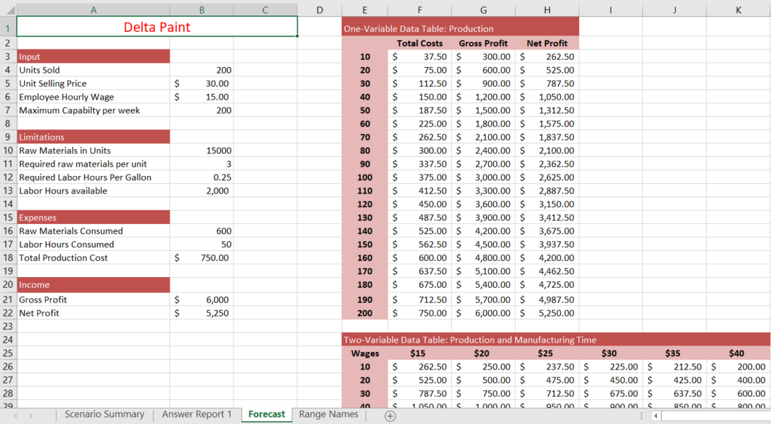
Create appropriate range names for Total Production Cost (cell B18) and Gross Profit (cell B21) by selection, using the values in the left column.
3
Edit the existing name range Employee_Hourly_Wage to Hourly_Wages2018.
Note, Mac users, in the Define Name dialog box, add the new named range, and delete the original one.
4
Use the newly created range names to create a formula to calculate Net Profit (in cell B22).
5
Create a new worksheet labeled Range Names, paste the newly created range name information in cell A1, and resize the columns as needed for proper display.
6
On the Forecast sheet, start in cell E3. Complete the series of substitution values ranging from 10 to 200 at increments of 10 gallons vertically down column E.
7
Enter references to the Total_Production_Cost, Gross_Profit, and Net Profit cells in the correct locations (F2, G2, and H2 respectively) for a one-variable data table. Use range names where indicated.
8
Complete the one-variable data table in the range E2:H22 using cell B4 as the column input cell, and then format the results with Accounting Number Format with two decimal places.
9
Apply custom number formats to make the formula references appear as descriptive column headings. In F2, Total Costs; in G2, Gross Profit, in H2, Net Profit. Bold and center the headings and substitution values.
10
Copy the number of gallons produced substitution values from the one-variable data table, and then paste the values starting in cell E26.
11
Type $15 in cell F25. Complete the series of substitution values from $15 to $40 at $5 increments.
12
Enter the reference to the net profit formula in the correct location for a two-variable data table.
13
Complete the two-variable data table in the range E25:K45. Use cell B6 as the Row input cell and B4 as the Column input cell. Format the results with Accounting Number Format with two decimal places.
14
Apply a custom number format to make the formula reference appear as a descriptive column heading Wages. Bold and center the headings and substitution values where necessary.
15
Create a scenario named Best Case, using Units Sold, Unit Selling Price, and Employee Hourly Wage (use cell references). Enter these values for the scenario: 200, 30, and 15.
16
Create a second scenario named Worst Case, using the same changing cells. Enter these values for the scenario: 100, 25, and 20.
17
Create a third scenario named Most Likely, using the same changing cells. Enter these values for the scenario: 150, 25, and 15.
18
Generate a scenario summary report using the cell references for Total Production Cost and Net Profit.
19
Load the Solver add-in if it is not already loaded. Set the objective to calculate the highest Net Profit possible.
20
Use the units sold as changing variable cells.
21
Use the Limitations section of the spreadsheet model to set a constraint for raw materials. Use cell references to set constraints.
22
Set a constraint for labor hours. Use cell references to set constraints.
23
Set a constraint for maximum production capability. Use cell references to set constraints.
24
Solve the problem. Generate the Answer Report and Keep Solver Solution.
25
Create a footer on all four worksheets with your name on the left side, the sheet name code in the center, and the file name code on the right side.
26
Save and close the file. Based on your instructor’s directions, submit exploring_e06_grader_Capstone.xlsx.
Step
Instructions
1
Open exploring_e07_grader_h1_Apartment.xlsx and save it as exploring_e07_grader_h1_Apartment_LastFirst.
2
In cell G8 in the Summary worksheet, insert a date function to calculate the number of years between 1/1/2018 in cell H2 and the last remodel date in the Last Remodel column (cell F8). Use relative and mixed references correctly. Copy the function to the range G9:G57. Unit 101 was last remodeled 13.75 years ago. Ensure that the function you use displays that result.
3
In cell H8, insert a nested logical function to display the required pet deposit for each unit. If the unit has two or more bedrooms (C8) AND was remodeled less than 10 years ago (cell H3), the deposit is $275 (cell H4); if not, the deposit is $200 (cell H5). Use relative and mixed references correctly. The pet deposit for Unit 101 is $200.
4
In cell I8, enter a nested logical function to display Need to Remodel if the apartment is unoccupied (No) AND was last remodeled more than 10 years ago (H3). For all other apartments, display No Change. Although Unit 101 was last remodeled over 10 years ago, the recommendation is No Change because the unit is occupied.
5
Copy the functions in the range H8:I8 to the range H9:I57.
6
In cell B3 insert a nested MATCH function within an INDEX function that will look up the rental price in column D using the apartment number referenced in cell B2. With 101 entered in cell B2, the lookup function displays $950.00.
7
In the Database sheet, enter conditions in the criteria range for unoccupied two- and three-bedroom apartments that need to be remodeled. Enter criteria as text only, without use of quotation marks. Be sure to enter the criteria separately in rows 3 and 4.
8
Apply an advanced filter based on the criteria range (A2:H4). Filter the existing database (range A15:H65) in place. Nine apartments meet the advanced filter conditions.
9
In cell C8, use the DCOUNTA database function to calculate the number of apartments that need to be remodeled based on the advanced filter you created.
10
In cell C9, enter a database function to calculate the total value of monthly rent lost for the apartments that need to be remodeled based on the advanced filter you created.
11
In cell C10, enter a database function to display the date of the apartment that had the oldest remodel date based on the filtered data. Format the result with Short Date format.
12
In the Loan sheet, insert formulas in the range E2:E4 to calculate the loan amount, the number of payment periods, and the monthly interest rate, respectively. Use cell references in all formulas.
13
In cell E5, enter a financial function to calculate the monthly payment. In cell E6, insert a financial function to calculate the cumulative total interest paid throughout the loan. Make sure the results display as positive numbers.
14
In cell C11, enter a formula to reference the date stored in cell B7. Insert a nested function in cell C12 to calculate the date for the next payment. Nest the YEAR, MONTH, and DAY functions within the DATE function. Add 1 to the month result. Copy the function to the range C13:C34.
15
In cell D11, enter a formula to reference the value stored in cell E2. Insert a formula in cell D12 that references the ending balance for the previous payment row (G11). Copy the formula in D12 to the range D13:D34.
16
In cell E11, enter a financial function to calculate the interest paid. Copy the formula to the range E12:E34. The result should be a positive value.
17
In cell F11, enter a financial function to calculate the principal payment. Copy the function to the range F12:F34. The result should be a positive value.
18
In cell G11, enter a formula to calculate the ending balance. Copy the formula to the range G12:G34. Adjust the width of column G, if needed, to display the values. Select the range D11:G34 and apply Accounting Number Format.
19
In cell I4 insert a financial function to calculate the present value of the total monthly rent you will collect for the 8 units for 30 years. Use the number of periods and monthly rate in the Summary Calculations section and the cell references in the What If section. The result should be a positive value.
20
In the Loan sheet, set 0.5″ left and right margins and repeat row 10 on all pages.
21
Save and close the workbook, and submit the file as directed.
Leave a Reply
- File Format (AG1): .accdb MS-Access database
- File Format (AG2):
- File Format(AG3):
- File Format (EG1):
- File Format (EG2):
- File Format (EG3):
- File Format (EG6): .xlsx MS-Excel
I would like to download AG2
Please check http://libraay.com/downloads/morris-arboretum/
I would like to downloag AG1
Please write to us for the same at info@libraay.com. The team shall make the solution available for you.