Office 2013 MyITLab MS-Excel Grader Credit Card Expenses
You started recording every credit card transaction so that you can analyze your monthly expenses. You used an Excel worksheet to track dates, places, categories, and amounts. Because you are a consultant who travels periodically, you also have business expenses. You included a column to indicate the business-related transactions. Now you need to convert the data to a table, sort and filter the data to analyze it, and apply conditional formatting to apply a visual effect for further analysis.
Instructions:
For the purpose of grading the project you are required to perform the following tasks:
| Step | Instructions | Points Possible |
| 1 | Start Excel. Open the downloaded Excel file named exploring_e04_grader_a1.xlsx. | 0 |
| 2 | In the Dining Out worksheet, convert the data to a table. Apply Table Style Light 14. | 10 |
| 3 | Remove duplicate rows in the Dining Out worksheet. | 5 |
| 4 | Sort the table by Description in alphabetical order, then by Store in alphabetical order, and then by Amount from the smallest to the largest. | 10 |
| 5 | Filter the records to show personal (i.e., non-business) lunch and dinner expenses. | 10 |
| 6 | Display the Total Row. In cell D48, select the function to total the Amount values. In cell E48, do not show a total. | 10 |
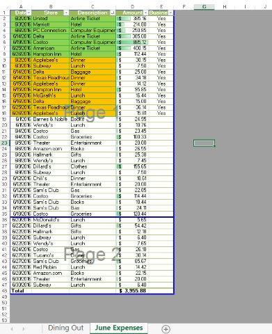
| 7 | In the June Expenses worksheet, apply the conditional formatting style that displays a Green Data Bar Gradient Fill in the range D2:D47. | 5 |
| 8 | Create a conditional formatting rule with these specifications to the range A2:C47: • Formula to determine which cells to format • Formula: =(AND(argument1,argument2)) where argument1 compares $D2 to see if it is greater than or equal to 100 and argument 2 compares $E2 to see if the text is “Yes”. • Light Green (Standard) fill color • Green border color • Outline preset border style |
10 |
| 9 | Create a conditional formatting rule with these specifications to the range A2:C47: • Formula to determine which cells to format • Formula: =(AND(argument1,argument2)) where argument1 compares $D2 to see if it is less than 100 and argument 2 compares $E2 to see if the text is “Yes”. • Orange (Standard) fill color • Green border color • Outline preset border style |
10 |
| 10 | Create a custom color sort for the Description column with these specifications: • Sort on cell color to display the Light Green (Standard) fill color on Top as the primary sort. • Sort on cell color to display the Orange (Standard) fill color on Top as the secondary sort. |
10 |
| 11 | Freeze the top row. | 5 |
| 12 | Set the Scale to Fit percentage to 115%. Display the worksheet in Page Break Preview and insert a page break so that row 36 starts on a new page. | 5 |
| 13 | Repeat the titles on row 1 on all pages. | 5 |
| 14 | Insert a custom footer with the text Exploring Series on the left side, the sheet name code in the center, and the file name code on the right side of the June Expenses worksheet. | 5 |
| 15 | Ensure that the worksheets are correctly named and placed in the following order in the workbook: Dining Out, June Expenses. Save the workbook. Close the workbook, and then exit Excel. Submit the workbook as directed. | 0 |
| Total Points | 100 |
- File Format: MS-Excel .xlsx
- Version: 2013