Office 2016 myITLab MS-Excel Grader EX16_XL_CH05_GRADER_CAP_AS – Travel Expenses 1.8
-----View all MS-Excel 2016 MyITLab Grader Digital Solution Download Files-----
-----Purchase MS-Excel 2016 MyITLab Grader Discounted Bundle Here-----
| Step | Instructions | Points Possible |
| 1 | Start Excel. Open the downloaded Excel file named exploring_e05_grader_a1_Expenses.xlsx. Save the workbook as exploring_e05_grader_a1_Expenses_LastFirst, replacing LastFirst with your own name. | 0 |
| 2 | On the Subtotals worksheet, use the Sort dialog box to sort the data by Employee and further sort by Category, both in alphabetical order. | 4 |
| 3 | Use the Subtotals feature to insert subtotal rows by Employee to calculate the total expense by employee. | 6 |
| 4 | Collapse the Donaldson and Hart sections to show only their totals. Leave the other employees’ individual rows displayed. | 5 |
| 5 | Use the Expenses worksheet to create a blank PivotTable on a new worksheet named Summary. Name the PivotTable Categories. | 8 |
| 6 | Use the Category and Expense fields, enabling Excel to determine where the fields go in the PivotTable. | 5 |
| 7 | Modify the Values field to determine the average expense by category. Change the custom name to Average Expense. | 4 |
| 8 | Format the Values field with Accounting number type. | 4 |
| 9 | Type Category in cell A3 and change the Grand Totals layout option to On for Rows Only. | 5 |
| 10 | Apply Pivot Style Dark 2 and display banded rows.
Note, depending upon the version of Office being used, the style name may be Light Blue, Pivot Style Dark 2. |
5 |
| 11 | Insert a slicer for the Employee field, change the slicer height to 2 inches and apply the Slicer Style Dark 5. Move the slicer below the PivotTable. Note, depending upon the version of Office being used, the style name may be Light Blue, Slicer Style Dark 5. |
6 |
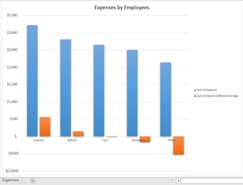
| 12 | Use the Expenses worksheet to create another blank PivotTable on a sheet named Totals. Add the Employee to the Rows and add the Expense field to the Values area. Sort the PivotTable from largest to smallest expense. | 10 |
| 13 | Change the name for the Expenses column to Totals and format the field with Accounting number format. | 6 |
| 14 | Insert a calculated field to subtract 2659.72 from the Expense field. Format the field with the custom name Above or Below Average and apply Accounting number format to the field. | 10 |
| 15 | Set 12.29 (approximate) as the width for column B and column C, change the row height of row 3 to 30, and apply word wrap to cell C3. | 4 |
| 16 | Create a clustered column PivotChart from the PivotTable. Move the PivotChart to a new sheet named Chart. Hide all field buttons in the PivotChart, if necessary. Note, Mac users, select the range A3:C8 in the PivotTable. On the Insert tab, click Column, and then click Clustered Column. Right-click, and from the shortcut menu, click Move Chart. |
10 |
| 17 | Add a chart title above the chart and type Expenses by Employee. Change the chart style to Style 14.
Note, Mac users, continue on to the next Step. |
0 |
| 18 | Apply 11 pt font size to the value axis and display vertical axis as Accounting with zero decimal places. | 4 |
| 19 | Create a footer on all worksheets with your name in the left section, the sheet name code in the center section, and the file name code in the right section. | 4 |
| 20 | Ensure that the worksheets are correctly named and placed in the following order in the workbook: Subtotals, Summary, Chart, Totals, Expenses. Save the workbook. Close the workbook and then exit Excel. Submit the workbook as directed. | 0 |
| Total Points | 100 |
-----View all MS-Excel 2016 MyITLab Grader Digital Solution Download Files-----
- File Format (Solution File): MS-Excel .xlsx
- Version: 2016
- File Format(Guide): .PDF