Office 2016 myITLab MS-Excel Grader EX16_XL_CH08_GRADER_CAP_AS – Job Satisfaction 1.6
-----View all MS-Excel 2016 MyITLab Grader Digital Solution Download Files-----
-----Purchase MS-Excel 2016 MyITLab Grader Discounted Bundle Here-----
-----View all MS-Excel 2016 MyITLab Grader Digital Solution Download Files-----
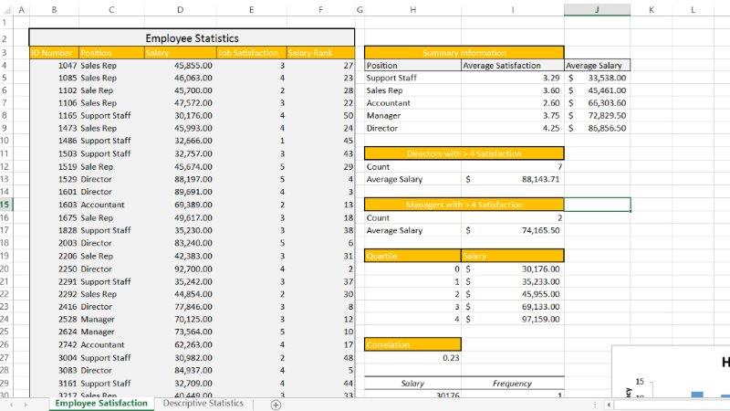
In this project, you will use Excel to perform statistical analysis of a cross-sectional sample of an employee satisfaction survey.
Instructions:
For the purpose of grading the project you are required to perform the following tasks:
| Step | Instructions | Points Possible |
| 1 | Download and open the file named exploring_e08_grader_a1.xlsx, and then save the file as exploring_e08_grader_a1_LastFirst, replacing LastFirst with your name. | 0 |
| 2 | Enter a conditional function in cell I5 to calculate average satisfaction for support staff (H5). Format the results with Number format and two decimal positions. | 6 |
| 3 | Use the fill handle in cell I5 to copy the function down through the range I6:I9. Be sure to use the appropriate mixed or absolute referencing before copying the functions. | 3 |
| 4 | Enter a function in cell J5 to calculate the average salary of all support staff (H5) in the survey. | 6 |
| 5 | Use the fill handle in cell J5 to copy the function down through the range J6:J9. Be sure to use the appropriate mixed or absolute referencing before copying the functions. | 3 |
| 6 | Enter a function in cell I12 to calculate the number of Directors in the survey that have a job satisfaction level of 4 or higher. | 6 |
| 7 | Enter a function in cell I13 to calculate the average salary of Directors in the survey that have a job satisfaction level of 4 or higher. | 6 |
| 8 | Adapt the process used in the previous two steps to calculate the total number and average salary of managers that have a job satisfaction of 4 or higher in cells I16 and I17. | 6 |
| 9 | Enter a function in cell F4 that calculates the rank of the salary in cell D4 against the range of salaries in the data set. | 6 |
| 10 | Use the fill handle to copy the function down column F. Be sure to include the appropriate absolute or mixed cell references before copying the functions. | 5 |
| 11 | Enter a function in cell I20 to calculate the minimum Quartile value in the list of salaries. | 6 |
| 12 | Use the fill handle to complete the remaining quartile values in cell range I21:I24. Be sure to include the appropriate absolute or mixed cell references before copying the functions. | 5 |
| 13 | Enter a function in cell H27 to calculate the correlation of column D and E. | 12 |
| 14 | Format the result as Number Format with two decimal positions. | 5 |
| 15 | If necessary, display the Analysis ToolPak. Run a Data Analysis with descriptive statistics. Complete the input criteria using the salary data in the range D4:D53. Set the Output functions to display on a new worksheet. Set the output as Summary statistics. | 12 |
| 16 | Name the newly created worksheet Descriptive Statistics. | 3 |
| 17 | On the Employee Satisfaction worksheet, run a Data Analysis histogram. Use the salaries in the range D4:D53 as the input range. Use the quartiles in the range I20:I24 as the bin range. Output the data in cell H29. Include a chart with the output. | 10 |
| 18 | Move the Employee Satisfaction worksheet to display first in the workbook, if necessary. Ensure that the worksheets are correctly named and placed in the following order in the workbook: Employee Satisfaction; Descriptive Statistics. Save the workbook. Close the workbook and then exit Excel. Submit the workbook as directed. | 0 |
| Total Points | 100 |
- File Format (Solution File Only): MS-Excel .xlsx
- Version: 2016
- File Format(Guide): .PDF