Office 2016 MyITLab MS-Excel Grader Final Exam
-----View all MS-Excel 2016 MyITLab Grader Digital Solution Download Files-----
-----Purchase MS-Excel 2016 MyITLab Grader Discounted Bundle Here-----
-----View all MS-Excel 2016 MyITLab Grader Digital Solution Download Files-----
You are planning on taking a vacation abroad later this year. You have designed a currency converter so you can determine how much money you need to take into each country. Once you return, you will be purchasing a new boat, so you are also working on an amortization table in order to adjust your budget. Of course, you are working on these tasks in your spare time at work as an administrative assistant for the CIS Department, where you are working on several worksheets to evaluate faculty data.
Steps to Perform:
| Step | Instructions | Points Possible |
| 1 | Open Excel, and then open the downloaded file final_exam.xlsx. | 0 |
| 2 | On the Currency Exchange worksheet, format the title International Travel Currency Converter as bold with 14 pt font. Merge and center the range A1:D1. | 5 |
| 3 | Use the VLOOKUP function, the data on the Currency Table worksheet, and appropriate relative and absolute cell references to display the country’s currency name in its respective cell in row 5. For example, the country currency for Germany should be Euro. | 5 |
| 4 | Use the VLOOKUP function and the Currency Table to calculate the amount due based on each country’s exchange rate in each country’s respective cell in row 6. Be sure to use absolute cell references where necessary. Change the monetary symbol accordingly for each conversion (using the Euro € 123 format for Germany). | 5 |
| 5 | Format the range A3:D4 with Yellow fill (under Standard Colors) and a thick outside border. Format the range A5:D6 with Green fill (under Standard Colors) and a thick outside border. | 5 |
| 6 | Format the Currency Exchange worksheet to print in landscape orientation, with the data centered horizontally. Insert a header with the current date (using the &[Date] tag) inserted on the left and your name on the right side. | 5 |
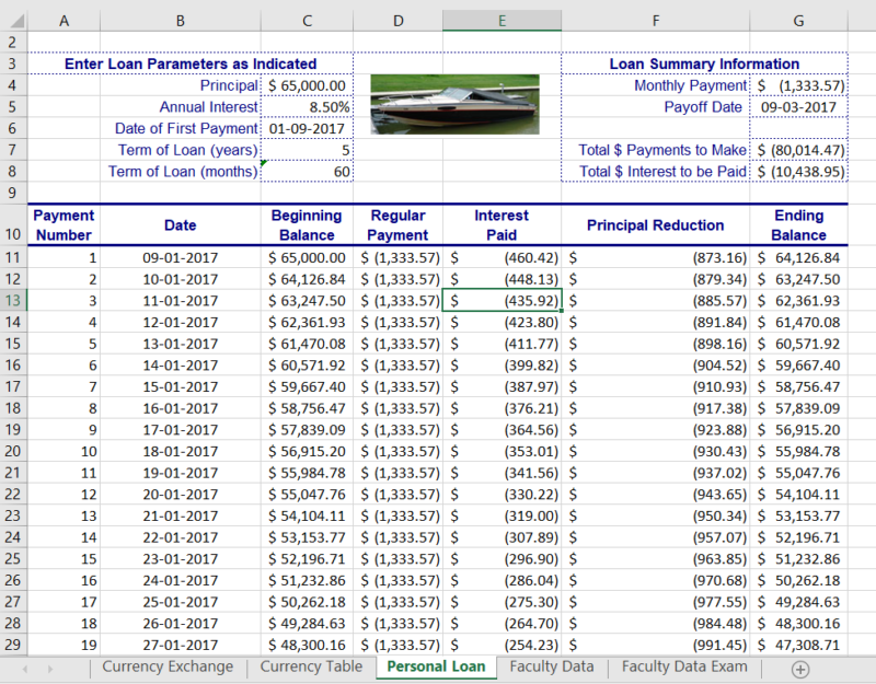
| 7 | Display the Personal Loan worksheet. Insert a formula in cell C8 to calculate the total number of payments for the loan using relative cell references. | 5 |
| 8 | In cell G4, use the PMT function to calculate the monthly payment for the loan. Be sure to use relative cell references. The function should return a negative value. | 5 |
| 9 | In cell A11, enter 1 as the first payment number and in cell B11, enter 9/1/2017 as the first payment date. In cell C11, insert a relative reference to the loan amount and in cell D11, insert an absolute reference to the monthly payment amount. In cell E11, use the IPMT function to calculate the interest paid for the first month (use absolute references where appropriate and leave the result as a negative value). In cell F11, use the PPMT function to calculate the principal payment for the first month (use absolute references where appropriate and leave the result as a negative value). In cell G11, use relative references to add the values in cells C11 and F11. | 10 |
| 10 | Select the range D11:G11, and then use the fill handle to copy the functions to row 12. In cell A12, enter 2 as the second payment number and in cell B12, enter 10/1/2017 as the second payment date. In cell C12, insert a relative reference to the ending balance in cell G11. Select the range A11:B12, and then use the fill handle to complete the columns through row 70. Select the range C12:G12, and then use the fill handle to complete the amortization table. | 5 |
| 11 | In cell G5, reference the payoff date of the loan (the date of the last payment). Be sure to use a relative reference to the cell containing the date. | 5 |
| 12 | Use the SUM function in cell G7 to calculate the total amount paid over the course of the loan. Use the SUM function in cell G8 to calculate the total interest paid over the course of the loan. Both functions should return negative values. | 5 |
| 13 | Format all cells containing dollar amounts to Accounting format, if necessary. Format all cells containing dates to display the date using the default Date format and center the dates in the cells. | 5 |
| 14 | Create a copy of the Faculty Data worksheet to the right of the last sheet tab. Rename the new worksheet as Faculty Data Exam. | 5 |
| 15 | On the Faculty Data Exam worksheet, sort the table data by Department, then by Rank, both in ascending order. Insert a comment in cell J3 with the text Matching Rate Should Be Raised! | 5 |
| 16 | Use Find & Replace to replace all instances of Full with Full Professor in the Rank column (use Ctrl-F to display Find & Replace window). AutoFit the width of column D. | 5 |
| 17 | In cell J3, use the IF function to calculate the retirement matching for each faculty member participating in the retirement plan. For participating members, the function should multiply their salary by the retirement matching percentage. For all other members, the function should return 0. Be sure to make the reference to cell J1 an absolute reference in the function. Use the fill handle to copy the function down through the column. Apply the currency format to the values. | 5 |
| 18 | Using the data in A2:J8, insert a PivotTable starting in cell A10. Add Department to the Rows, Gender to the Columns and Salary to the Values area. Format salaries to the Accounting format with no decimal places. | 5 |
| 19 | Display the Faculty Data worksheet, and then create a table with headers using the data in the range A2:J8. Change the name of the table to FacultyData. Sort in ascending order by YearHired, and then filter the table to show only those faculty hired between 1982 and 1985. | 5 |
| 20 | Using the filtered data results, select the nonadjacent ranges of C2:C5 and H2:H5 then insert a 2-D pie chart. Move and resize the pie chart so that it fills the range A10:E21. Change the title of the pie chart to Salary for College of Business Hires 1982-1985. Change the font of the chart title to 10.5 pt. | 5 |
| 21 | Save the workbook. Ensure that the worksheets are in the following order: Currency Exchange, Currency Table, Personal Loan, Faculty Data, and Faculty Data Exam. Save the workbook, exit Excel, and then submit your file as directed by your instructor. | 0 |
| Total Points | 100 |
- File Format (Solution File): MS-Excel .xlsx
- Version: 2016
- File Format(Guide): .PDF