Office 2013 MyITLab MS-Excel Grader Statistical Functions
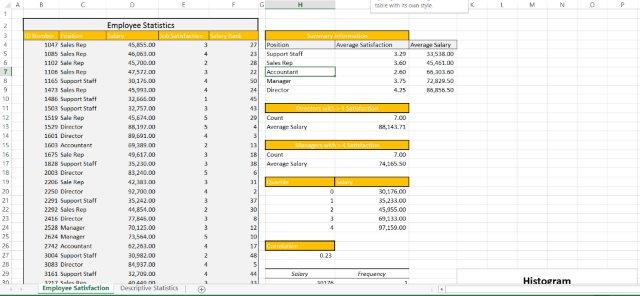
In the following project, you will use excel to perform statistical analysis of a cross section sample of an employee satisfaction survey.
Instructions:
For the purpose of grading the project you are required to perform the following tasks:
| Step | Instructions | Points Possible |
| 1 | Download and open the file named exploring_e08_grader_h1, and then save the file as exploring_e08_grader_h1_LastFirst, replacing “LastFirst” with your name. | 0 |
| 2 | Enter a conditional function in cell I5 to calculate average satisfaction for support staff (H5). Format the results with Number format and two decimal positions. | 6 |
| 3 | Use the fill handle in cell I5 to copy the function down through the range I6:I9. Be sure to use the appropriate mixed or absolute referencing before copying the functions. | 3 |
| 4 | Enter a function in cell J5 to calculate the average salary of all support staff (H5) in the survey. | 6 |
| 5 | Use the fill handle in cell J5 to copy the function down through the range J6:J9. Be sure to use the appropriate mixed or absolute referencing before copying the functions. | 3 |
| 6 | Enter a function in cell I12 to calculate the number of Directors in the survey that have a job satisfaction level of 4 or higher. | 6 |
| 7 | Enter a function in cell I13 to calculate the average salary of Directors in the survey that have a job satisfaction level of 4 or higher. | 6 |
| 8 | Adapt the process used in the previous two steps to calculate the total number and average salary of managers that have a job satisfaction of 4 or higher in cells I16 and I17. | 6 |
| 9 | Enter a function in cell F4 that calculates the rank of the salary in cell D4 against the range of salaries in the data set. | 6 |
| 10 | Use the fill handle to copy the function down column F. Be sure to include the appropriate absolute or mixed cell references before copying the functions. | 5 |
| 11 | Enter a function in cell I20 to calculate the minimum Quartile value in the list of salaries. | 6 |
| 12 | Use the fill handle to complete the remaining quartile values in cell range I21:I24. Be sure to include the appropriate absolute or mixed cell references before copying the functions. | 5 |
| 13 | Enter a function in cell H27 to calculate the correlation of column D and E. | 12 |
| 14 | Format the results as Number Format with two decimal positions. | 5 |
| 15 | Click the DATA tab and select Data Analysis. Select Descriptive Statistics and click OK. Complete the input criteria using the salary data in column D. Set the Output functions to display on a new worksheet. (Hint: be sure to output Summary Statistics). | 12 |
| 16 | Name the newly created worksheet Descriptive Statistics. | 3 |
| 17 | Click the DATA tab and select Data Analysis. Select Histogram and click OK. Use the salaries in column D as the input range. Use the quartiles in the range I20:I24 as the bin range. Output the data in cell H29. Be sure to include a chart with the output. | 10 |
| 18 | Move the Employee Satisfaction worksheet to display first in the workbook. Ensure that the worksheets are correctly named and placed in the following order in the workbook: Employee Satisfaction; Descriptive Statistics. Save the workbook. Close the workbook and then exit Excel. Submit the workbook as directed. | 0 |
| Total Points | 100 |
- File Format: MS-Excel .xlsx
- Version Used: 2013

