Office 2013 MyITLab MS-Excel Grader Fine Art Dealer
You are an analyst for an authorized Greenwich Workshop® fine art dealer (www.greenwichworkshop.com). Customers are especially fond of James C. Christensen’s art. The Subtotals worksheet contains a list of artwork released in 2010-2012. You want to calculate subtotals by Type of art (e.g. Limited Edition Canvas) for Issue Price and Est. Price. The Art worksheet contains artwork from 2004-2006. Studying this data will help you discuss value trends with art collectors.
Instructions:
For the purpose of grading the project you are required to perform the following tasks:
| Step | Instructions | Points Possible |
| 1 | Start Excel. Open the downloaded Excel file named exploring_e05_grader_h1_start.xlsx. | 0 |
| 2 | In the Subtotals worksheet, sort the data by Type and then by Name of Art, both in alphabetical order.
Hint: On the DATA tab, in the Sort & Filter group, click Sort. |
5 |
| 3 | In the Subtotals worksheet, use the Subtotals feature to identify the highest Issue Price and Est. Value, for each different value of Type.
Hint: On the DATA tab, in the Outline group, click Subtotal. |
5 |
| 4 | Use the Art worksheet to create a blank PivotTable on a new worksheet named PivotTable. | 5 |
| 5 | Include the Type, Release Date, and Issue Price fields in the PivotTable. Remove the Release Date field and add the Est. Value field to the PivotTable. | 5 |
| 6 | Modify the two VALUES fields to determine the Average Issue Price and Average Est. Value instead of the Sum. Change the custom name to Average Issue Price and Average Est. Value, respectively. | 10 |
| 7 | Format the two VALUES fields with Accounting Number type with zero decimal places. | 5 |
| 8 | Insert a calculated field on the right side of the PivotTable that displays the difference between the Est. Value and Issue Price, as a percentage of Issue Price.
Hint: On the ANALYZE tab, in the Calculations group, click Fields, Items & Sets, and then click Calculated Field. In the Insert Calculated Field, type: |
5 |
| 9 | Format the calculated field with Percent type with two decimal places. Use the custom name Percentage Change. | 5 |
| 10 | Type Type in cell A3 and Overall Averages in the cell containing the text Grand Total. | 5 |
| 11 | Set a filter to display only sold-out art (indicated by Yes). | 5 |
| 12 | Apply Pivot Style Medium 5, display banded columns, and display banded rows. | 10 |
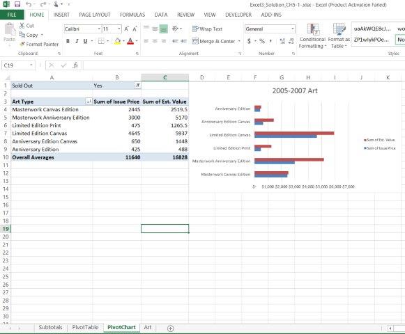
| 13 | Use the Art worksheet to create a PivotChart on a new sheet named PivotChart. Change the chart type to Clustered Bar. | 5 |
| 14 | Include the Type, Issue Price, and Est. Value fields. Set a filter to display only sold-out art (indicated by Yes) for the PivotChart. | 10 |
| 15 | Hide the field buttons in the PivotChart. Insert a chart title above the chart and type 2005-2007 Art. | 5 |
| 16 | Format the value axis with Accounting with zero decimal places. Apply 8-pt size to the category axis and value axis. Apply 7-pt size to the legend. | 5 |
| 17 | Adjust the size of the PivotChart for the range D1:K14. | 5 |
| 18 | Sort the data in the PivotChart’s PivotTable in reverse alphabetical order by Type. Type Art Type in cell A3 and type Overall Averages in the cell containing the text Grand Total. | 5 |
| 19 | Ensure that the worksheets are correctly named and placed in the following order in the workbook: Subtotals, PivotTable, PivotChart, Art. Save the workbook. Close the workbook and then exit Excel. Submit the workbook as directed. | 0 |
| Total Points | 100 |
Leave a Reply
- File Format: Microsoft Excel .xlsx
- Version Used: 2013
- Custom Solution Available: Yes


How do i access this purchase?
Thank you for your message.
The solution files are mailed to your E-Mail ID immediately after the purchase. We suggest you to also check your Junk/Spam folders for a mail with subject line “You just made a purchase”. If you still do not get access to the solution files, please write to info@libraay.com.
Team Libraay