Office 2013 MyITLab MS-Excel Grader Mountain View Realty
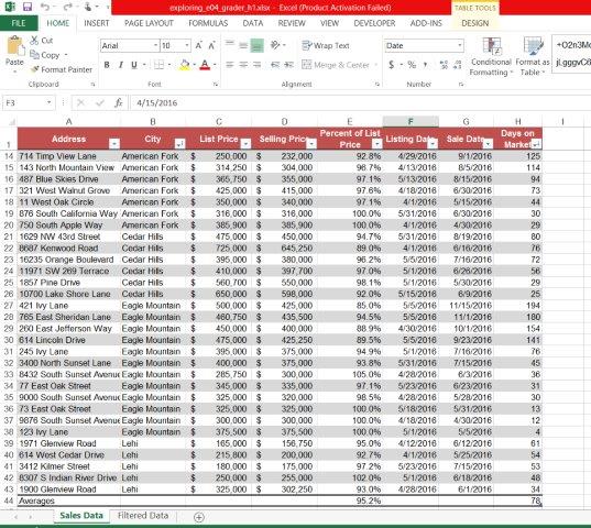
A coworker developed a spreadsheet listing houses listed and sold during the past several months. She included addresses, location, list price, selling price, listing date, and date sold. You need to convert the data to a table. You will manage the large worksheet, prepare the worksheet for printing, sort and filter the table, include calculations, and format the table.
Instructions:
For the purpose of grading the project you are required to perform the following tasks:
| Step | Instructions | Points Possible |
| 1 | Start Excel. Open the downloaded file named exploring_e04_grader_h1.xlsx. | 0 |
| 2 | In the Sales Data worksheet, freeze the top row.
Hint: On the VIEW tab, in the Window group, click Freeze Panes and then click Freeze Top Row. |
5 |
| 3 | In the Sales Data worksheet, convert the data to a table and apply Table Style Medium 17. | 6 |
| 4 | In the Sales Data worksheet, remove duplicate records in the table.
Hint: |
5 |
| 5 | In the Sales Data worksheet, insert a new field to the right of the Selling Price field. Name the new field Percent of List Price. | 6 |
| 6 | In the Sales Data worksheet, create a formula in cell E2 with structured references to calculate the percent of the list price. Format the field with Percent Style with one decimal place in the range E2:E43.
`Hint: |
6 |
| 7 | In the Sales Data worksheet, insert a new field to the right of the Sale Date field. Name the new field Days on Market. Create a formula with structured references to calculate the number of days on the market.
Hint: |
6 |
| 8 | In the Sales Data worksheet, add a total row to display the average percent of list price and average number of days on market. Apply the General number format to the average number of days on market as a whole number. Type Averages in cell A44. | 10 |
| 9 | In the Sales Data worksheet, sort the table by City in alphabetical order and add a second level to sort by Days on Market with the houses on the market the longest at the top within each city.
Hint: |
8 |
| 10 | In the Sales Data worksheet, select the Listing Date and Sale Date fields and set a column width of 11.00. Wrap the column labels in the range E1:H1. | 6 |
| 11 | In the Sales Data worksheet, repeat the field names on all pages.
Hint: On the PAGE LAYOUT tab, in the Page Setup group, click Print Titles. |
5 |
| 12 | Display the Sales Data worksheet in Page Break Preview and move the page break to occur between rows 26 and 27, and then change back to Normal view.
Hint: To display Page Break Preview, on the VIEW tab, in the Workbook Views group, click Page Break Preview. To insert the page break, click cell A27 and on the PAGE LAYOUT tab, in the Page Setup group, click Breaks. |
5 |
| 13 | Display the Filtered Data worksheet. Convert the table to a range of data. | 5 |
| 14 | Filter the data to display the cities of Alpine, Cedar Hills, and Eagle Mountain.
Hint: |
6 |
| 15 | Filter the data to display records for houses that were on the market 30 days or more. | 5 |
| 16 | Apply the 3 Arrows (Colored) icon set to the days on market values.
Hint: On the HOME tab, in the Styles group, click Conditional Formatting and then point to Icon Sets. |
5 |
| 17 | Apply the Light Blue Data Bar conditional formatting in the Gradient Fill section to the selling prices.
Hint: On the HOME tab, in the Styles group, click Conditional Formatting and then point to Data Bars. |
5 |
| 18 | Create a new conditional format that applies Yellow fill (fourth color in the bottom row) and bold font to values that are higher than 98% for the Percent of List Price column. | 6 |
| 19 | Ensure that the worksheets are correctly named and placed in the following order in the workbook: Sales Data, Filtered Data. Save the workbook. Close the workbook and then exit Excel. Submit the workbook as directed. | 0 |
| Total Points | 100 |
- File Format: Microsoft Excel .xls
- Version Used: 2013
- Custom Solution Available: Yes

