Office 2016 MyITLab MS-Excel Grader EX16_XL_CH02_GRADER_CAP_HW – Inland Jewelers 1.12 / Exp19_Excel_Ch02_CapAssessment_Inland_Jewelers
-----View all MS-Excel 2016 MyITLab Grader Digital Solution Download Files-----
-----Purchase MS-Excel 2016 MyITLab Grader Discounted Bundle Here-----
-----View all MS-Excel 2016 MyITLab Grader Digital Solution Download Files-----
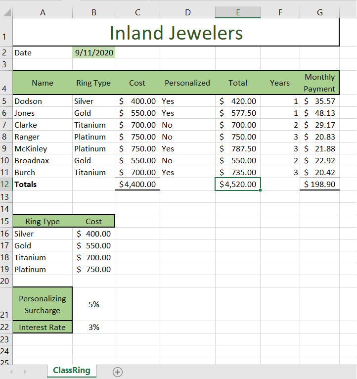
You are an account manager for Inland Jewelers, a regional company that makes custom class rings for graduating seniors. Your supervisor requested a workbook to report on new accounts created on payment plans. The report should provide details on total costs to the student as well as payment information. Each ring financed has a base price that can fluctuate based on ring personalization.
Steps to Perform:
| Step | Instructions | Points Possible |
| 1 | Start Excel. Download and open the file named exploring_e02_grader_h1.xlsx. | 0 |
| 2 | Insert a function in cell B2 to display the current date from your system. | 10 |
| 3 | With cell B2 selected, set the width of column B to AutoFit. | 2 |
| 4 | Insert a VLOOKUP function in cell C5 to display the ring cost for the first student. | 14 |
| 5 | Copy the formula from cell C5 to the range C6:C11. | 6 |
| 6 | Apply Accounting number format to the range C5:C11. | 3 |
| 7 | Insert an IF function in cell E5 to calculate the total due. If the student has chosen to personalize the ring, there is an additional charge of 5% located in cell B21 that must be applied; if not, the student only pays the base price. Use appropriate relative and absolute cell references. | 14 |
| 8 | Copy the formula from cell E5 to the range E6:E11. | 6 |
| 9 | Apply Accounting number format to the range E5:E11. | 3 |
| 10 | Insert a function in cell G5 to calculate the first student’s monthly payment, using appropriate relative and absolute cell references. | 14 |
| 11 | Copy the formula from cell G5 to the range G6:G11. | 7 |
| 12 | Apply Accounting number format to the range G5:G11. | 3 |
| 13 | Calculate totals in cells C12, E12, and G12. | 7 |
| 14 | Apply Accounting number format to the cells C12, E12, and G12, if necessary. | 2 |
| 15 | Set 0.3” left and right margins and ensure the page prints on only one page. | 5 |
| 16 | Insert a footer with your name on the left side, the sheet name in the center, and the file name on the right side. | 4 |
| 17 | Save the workbook. Close Excel. Submit the file as directed by your instructor. | 0 |
| Total Points | 100 |
- File Format (Solution File): .xlsx
- Version: 2016
- File Format (Guide): .PDF

