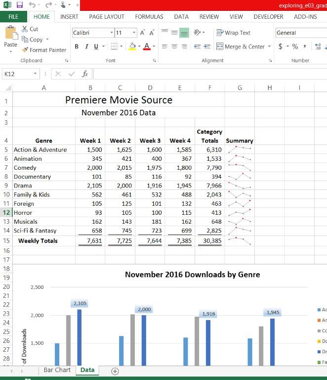
Office 2013 MyITLab MS-Excel Grader Premiere Movie Source
You are an assistant manager at Premiere Movie Source, an online company that enables customers to download movies for a fee. You need to track movie download sales by genre. You gathered the data for November 2016 and organized it in an Excel workbook. You are ready to create charts to help represent the data so that you can make a presentation to your manager later this week.
Instructions:
For the purpose of grading the project you are required to perform the following tasks:
| Step | Instructions | Points Possible |
| 1 | Start Excel. Open the downloaded Excel file named exploring_e03_grader_h1.xlsx. | 0 |
| 2 | Set chart filters to remove the Category Totals and the Weekly Totals.
Hint: Click the Chart Filters button to the right of the column chart. |
6 |
| 3 | Position and size the chart to fill the range A18:K37.
Hint: Click and drag to position the chart. Use the sizing handles to size the chart. |
6 |
| 4 | Change the row and column orientation so that the weeks appear in the category axis and the genres appear in the legend.
Hint: On the DESIGN tab, in the Data group, click the Switch Row/Column button. |
5 |
| 5 | Add a value axis title and type Number of Downloads. Apply Black, Text 1 font color to the value axis title.
Hint: To add the axis title, click the Chart Elements button to the right of the chart. Point to Axis Titles, and click the Axis Titles arrow. To format the title, on the HOME tab, use the tools in the Font group. |
6 |
| 6 | Move the legend to the right side of the chart and drag the bottom of the chart area down to cover row 37, if necessary.
Hint: To move the legend, click the Chart Elements button to the right of the chart. Point to Legend, and click the Legend arrow. To resize the chart, use the sizing handles. |
5 |
| 7 | Select the Drama data series and add data labels in the Outside End position. Add a default Gradient fill to the data labels. | 6 |
| 8 | Click cell G5 and insert Line Sparklines for the weekly data for each category and the weekly totals, but do not include the category totals for the data range. The location range should be G5:G15.
Hint: On the INSERT tab, in the Sparklines group, click Line. |
8 |
| 9 | Apply the Sparkline Style Accent 3, (no dark or light) sparkline style. | 4 |
| 10 | Show the high point and markers for the sparklines. Change the high point marker color to Red.
Hint: On the DESIGN tab, use the tools in the Show group to display the points. To change the color of the marker, in the Styles group, click Marker Color. |
6 |
| 11 | Select the range A4:E14. Create a stacked bar chart. Move the chart to new sheet. Type Bar Chart for the sheet name. | 6 |
| 12 | Add a chart title above the bar chart and type November 2016 Weekly Downloads. Apply bold and Blue, Accent 5 font color to the bar chart title.
Hint: Select the Chart Title placeholder, type the title text in the Formula Bar, and press ENTER. To format the chart title, on the HOME tab, use the tools in the Font group. |
8 |
| 13 | Apply 11 pt font size to the category axis, value axis, and the legend for the bar chart. | 6 |
| 14 | Use the Axis Options to display the value axis in units of Thousands, set the Major Units to 500, apply the Number format with 1 decimal place for the bar chart.
Hint: Double click the value axis labels. In the Format Axis pane, select Axis Options at the top of the pane. |
10 |
| 15 | Use the Axis Options to format the category axis so that the category labels are in reverse order.
Hint: |
4 |
| 16 | Create a footer on each worksheet with the text Exploring Series on the left side, the sheet name code in the center, and the file name code on the right side.
Hint: On the INSERT tab, in the Text group, click Header & Footer. |
6 |
| 17 | Apply landscape orientation for the Data worksheet. | 2 |
| 18 | Set 0.2 inch left, right, top, and bottom margins for the Data worksheet. Change the scaling so that the worksheet fits on only one page.
Hint: On the PAGE LAYOUT tab, in the Page Setup group, click the Page Setup Dialog Box Launcher. |
6 |
| 19 | Ensure that the worksheets are correctly named and placed in the following order in the workbook: Bar Chart, Data. Save the workbook. Close the workbook and then exit Excel. Submit the workbook as directed. | 0 |
| Total Points | 100 |
Leave a Reply
- File Format: Microsoft Excel .xls
- Version Used: 2013
- Custom Solution Available: Yes


This purchase did me no good since there were no instructions showing how you actually do each step so it was just a waste of $3 because I couldn’t even use it.
Thank you for your message.
Libraay is a platform offering student community with ready-to-use solution files as reference for their academic work. Currently we are not providing any tutorials and apologize for any inconvenience caused to you.
Libraay