Office 2013 MyITLab MS-Excel Grader Specialized Functions
In the following project, you will use Excel to perform calculations regarding rental properties. You will create a basic search, utilize database functions, and create an amortization table
Instructions:
For the purpose of grading the project you are required to perform the following tasks:
| Step | Instructions | Points Possible |
| 1 | Download and open the file named exploring_e07_grader_h1.xlsx, and then save the file as e07c2Apartment_LastFirst, replacing LastFirst with your name. | 0 |
| 2 | Insert functions in the Pet Deposit column of the Summary worksheet to calculate the required pet deposit for each unit. If the unit has two or more bedrooms and was remodeled after 2008 the deposit is $125, if not it is $75. | 10 |
| 3 | Enter nested functions in the Recommendation column to indicate Need to remodel if the apartment is unoccupied and was last remodeled before 2005. For all other apartments, display No change. | 10 |
| 4 | Type 101 in cell B2. | 4 |
| 5 | Insert a nested lookup function in cell E2 that will look up the rental price in column D using the apartment number referenced in cell B2. | 10 |
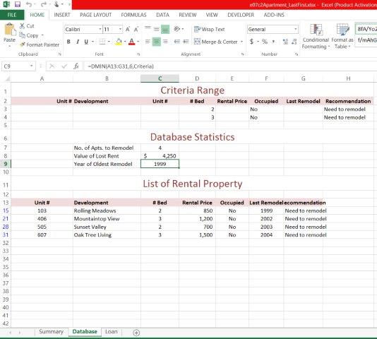
| 6 | Click the Database worksheet and enter conditions in the Criteria Range for unoccupied two- and three-bedroom apartments that need to be remodeled. | 10 |
| 7 | Perform an advanced filter based on the criteria range. Filter the existing database in place. | 10 |
| 8 | In cell C7, enter a DCOUNTA function to calculate the number of apartments to remodel. | 6 |
| 9 | In cell C8, enter a database function to calculate the total lost rent for the month. | 2 |
| 10 | Enter a database function to calculate the year of the oldest remodel in cell C9. | 2 |
| 11 | Click the Loan worksheet and enter 3/20/2015 in cell B7. | 2 |
| 12 | Insert a formula in cell E2 to calculate the loan amount based on the loan parameters in the input area. | 2 |
| 13 | Insert a formula in cell E3 to calculate the total number of periods. | 2 |
| 14 | Insert a formula in cell E4 to calculate the periodic monthly rate. | 2 |
| 15 | Insert a function in cell E5 to calculate the monthly payment. Ensure that the function returns a positive value. | 2 |
| 16 | In cell E6, insert a function to calculate the total interest paid on the loan. Ensure that the function returns a positive value.
Hint: To make CUMIPMT presented as positive numbers, place a ‘-‘ character in front of the function name, like this: =-CUMIPMT() This convention is repeated for =-CUMPRINC() But for: PMT(); IPMT(); and PPMT(), the ‘-‘ is placed in front of the pv amount, rather than the function name (like we did in Chp2). |
2 |
| 17 | Complete the loan amortization table for the first five payments only. In cell A11, enter 1. In cell B11, create a relative reference to cell B7 and in cell C11, create a relative reference to cell E2. Use the DATE function to complete the Payment Date column and financial functions for the Interest Paid and Principal Payment columns. In cell F11, enter =C11-E11. In cell C12, create a relative reference to cell F11. Note: Be sure to only complete the table through row 15.
Hint: |
18 |
| 18 | Create a footer with the sheet name code in the center, and the file name code on the right side of each worksheet. | 6 |
| 19 | Save the file making sure the worksheets are in the following order: Summary, Database, and Loan. Close Excel. Submit the file as directed. | 0 |
| Total Points | 100 |
- File Format: Microsoft Excel .xlsx
- Version Used: 2013
- Custom Solution Available: Yes

