Office 2013 MyITLab MS-Excel Grader Excel Final Exam Chapter 5-11
In this project, you will update a workbook to display bank transactions as a PivotTable. You will filter the PivotTable, format the values, display the values as calculations, and create a PivotChart using this data. Additionally, you will sort and subtotal data, create data tables, and use Goal Seek and Scenario Manager. You will format grouped worksheets, set up validation rules, and create functions. **Make sure you read the entire question, including hints, before you begin each section.
Instructions:
For the purpose of grading the project you are required to perform the following tasks:
| Step | Instructions | Points Possible |
| 1 | Start Excel. Open exploring_ecap_grader_c2_Transactions.xlsx and save the workbook as FinalExam_YourName | 0.000 |
| 2 | On the JuneTotals worksheet, sort the data in the range A3:E16 in ascending order by Category. At each change in Category, use the Sum function to add subtotals to the data in the Amount column. Accept all other defaults. Collapse the outline to show the grand total and Category subtotals only. | 4.500 |
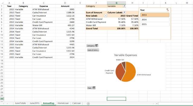
| 3 | Create a PivotTable in cell F1 on the AnnualExp worksheet using the data in the range A1:D17. Add the Expense field to the PivotTable as a row label; add the Amount field as the value; add the Year field as the column label. Change the format of the values in the PivotTable to accounting with no decimal places and set colums F:J to AutoFit Column Width. Use the Format Option in the Cells Category on the HOME tab to set columns F:J to AutoFit Column Width. | 8.000 |
| 4 | Add the Category field to the Report Filter area of the PivotTable. Filter the data so that only expenses in the Variable category are displayed. Display the values as percentages of the grand total.
Hint: To Display the values as percentages use ANALZYE > FIELD SETTINGS > SHOW VALUES AS > Select the appropriate setting |
4.000 |
| 5 | Insert a Year slicer in the worksheet and use the slicer to filter the data so that only data from 2013 is displayed. Change the height of the slicer to 2″ and then reposition it so that the top left corner aligns with the top left corner of cell I2. | 8.000 |
| 6 | Create a PivotChart in the worksheet based on the data in the PivotTable using the default Pie chart type. Change the chart title text to Variable Expenses and remove the legend. Add data labels to the outside end position displaying only the category names and leader lines. Reposition the chart so that the top left corner aligns with the top left corner of cell F13. | 4.000 |
| 7 | On the HomeLoan worksheet, in cell A10, enter a reference to the monthly payment from column B. Create a one-variable data table for the range A9:H10 using the interest rate from column B as the Row input cell. | 6.000 |
| 8 | On the HomeLoan worksheet, in cell A12, enter a reference to the monthly payment from column B. Create a two-variable data table in the range A12:H16, using the interest rate from column B as the Row input cell and the term in months from column B as the Column input cell. | 6.000 |
| 9 | On the HomeLoan worksheet, perform a goal seek analysis to determine what the down payment in column B needs to be if you want the monthly payment in column B to be 2000. Accept the solution. | 5.000 |
| 10 | On the HomeLoan worksheet, create a scenario named Maximum using cell references for the Retail Cost, Down Payment, Interest Rate and Term (in months) ( in that order) as the changing cells. Enter these values for the scenario: 280000, 24000, .075, and 360, respectively. Click OK and then close the dialogue box. DO NOT SELECT SHOW OR SUMMARY. You want the numbers from the Goal Seek Analysis to remain in your worksheet. Modify the numerical results to currency, two decimal places, if needed. | 5.000 |
| 11 | On the June2015 worksheet, in cell I7, sum the AMOUNTS if the purchase in column C is groceries; in cell I8, average the AMOUNTS if the purchase in column C is groceries; in cell I9, calculate the number of times groceries were purchased during the month. | 9.000 |
| 12 | On the June2015 worksheet, in cell I11, calculate the total amount spent on groceries using a credit card; in cell I12, calculate the average spent on groceries using a credit card; in cell I13, calculate the number of times groceries were purchased using a credit card during the month. | 9.000 |
| 13 | On the June2015 worksheet, in cell F7, nest an AND function within an IF function to determine if the transaction was paid using a credit card and the amount of the transaction is less than -100. If both conditions are met in the AND function, the function should return the text Flag. For all others, the function should return the text OK. Copy the function down through cell F24.
Hint: : You are looking for transactions that were purchased with a credit card and were over $100, you use -100 as the criteria because the transactions in the ledger are deductions from the checking account. Hint: Your results should show 1 flagged transaction. |
7.000 |
| 14 | On the June2015 worksheet, in cell E4, use the INDEX function to find the amount of the transaction when the position is entered in cell C4.
The position refers to the position in the ledger, assuming the first transaction 6/1/2015, Zachary Kaye, is in position 1. Your INDEX function should return a value 65.33 if 8 (Gas-N-Wash) is entered in field C4. Use A7:AE24 as the array argument. The column_num refers to the column number in the ledger (ex: The DATE would be column 1, PAYEE would be column 2). Both the Row_Num and Column_Num are required for this index function |
4.000 |
| 15 | On the June2015 worksheet,use an advanced filter to filter the data in the range A6:E24 using the criteria in the range A27:E28. Set the filter to copy the data to the range A31:E33 (be sure to select copy to another location).
In cell I17, use the DAVERAGE function to determine the average AMOUNT spent for transactions meeting the criteria in the range A27:E28. Use A6:F24 as the Database Range. |
6.000 |
| 16 | Group the June2015 and JuneTotals worksheets together. Fill the contents and formatting from cell A1 on the JuneTotals worksheet across the grouped worksheets. Ungroup the worksheets. In cell I19 on the June2015 worksheet, insert a 3D reference to cell E26 on the JuneTotals worksheet.
Hint: The reference to cell E26 allows changes to automatically occur in the June2015 worksheet if a change is made in E26 of the June Totals Worksheet, |
3.500 |
| 17 | On the June2015 worksheet, create a validation rule for the range D7:D24 to only allow values in the list from the range I21:I24. Create an error alert for the rule that will display after invalid data is entered. Using the Stop style, enter Invalid Entry as the title and Please select a valid method. ( include the period) as the error message. | 4.000 |
| 18 | On the CarLoan worksheet, in cell G10, use a function to calculate the cumulative principle paid on the car loan. Use appropriate absolute and/or relative references. Use the data in the range E4:E6 when entering the first three arguments in the function. Reference cell $A$10 as the start and A10 as then end period arguments. Enter 0 as the type argument. Modify the entire function (not individual arguments) to convert the results to a positive value. Copy the formula down through cell G19. Change the appropriate numerical data in the table to currency with two decimal places. | 3.000 |
| 19 | Apply the Retrospect theme to the workbook. Apply the cell style Accent1 to cells A3 and D3 on the CarLoan worksheet.
Hint : Use the THEMES section from the Page Layout Tab to apply the theme to the workbook; to apply accents to the individual cells use Cell Styles from the Cells category on the HOME tab. |
2.000 |
| 20 | Set the Title property to Personal Finances. | 2.000 |
| 21 | Delete the Stocks tab from the workbook. | 0.000 |
| 22 | Save the workbook. Ensure that the following worksheets are present (in this order): JuneTotals, June2015, Annual Exp, HomeLoan, CarLoan. Close the workbook, and then submit the file as directed. | 0.000 |
| 23 | CONGRATULATIONS ! You have completed ITEC 264!!! You are now an EXCEL expert. We covered a lot material this semester. You should be proud of yourself because you successfully completed the class ! | 0.000 |
| Total Points | 100.000 |
Leave a Reply to Jamie Cancel reply
- File Format: MS-Excel .xls
- Version: 2013
WOW! This tutor is great…I scored good score.
is this the current capstone myitlab chapters 5-11 final or is there an updated version?
Dear Jamie,
The solution is per the instructions mentioned on the webpage. You may mail your updated case to info@libraay.com if the instructions of the same doesn’t match with what is here.
Thank you.
Is there a video showing step by step how to complete each question? Or is it a final document of how the project should look like?
Hello, Thank you for your message. Currently, the purchased download shall contain only the final deliverable with all the steps solved, there is no video available.
It would be great if you guys had a step by step guide. The values vary in each class and even though this is the solution, the main goal is it to see the steps on how to get to the values and calculations. Missed that about the purchase. Hope you guys could update that. Other than that, thank you for the service!
Dear Miki MacCray, Thank you for your message. Our team is already working on tutorials and guides for all Grader cases. You shall soon see the website updated with that. Team Libraay.
Does this file have step by step instructions or just the final product of what the worksheets should look like?
Dear Bryan,
Currently Step-by-step How-to-Solve Tutorial guide is not available for this project. The download contains the solution for the case. Please contact us at info@libraay.com for any further assistance.
Team Libraay
Hello, I just purchased the file in the morning but it just gave me a 74% and I need the 90%.. Can you help me?
Dear Jose,
This may happen if you have a different starter file. Please write to us at info@libraay.com with complete details showing the marking sheets/errors found. Our team shall revert back to you at the earliest.
Team Libraay