Office 2016 myITLab MS-Excel Grader EX16_XL_COMP_GRADER_CAP_AS – Manufacturing 1.4 / 1.6
You have recently become the CFO for Beta Manufacturing, a small cap company that produces auto parts. As you step into your new position, you have decided to compile a report that details all aspects of the business, including: employee tax withholding, facility management, sales data, and product inventory. To complete the task, you will duplicate existing formatting, utilize various conditional logic functions, complete an amortization table with financial functions, visualize data with PivotTables, and lastly import data from another source.
Instructions:
For the purpose of grading the project you are required to perform the following tasks:
| Step | Instructions | Points Possible |
| 1 | Start Excel. Open eApp_Cap2_Manufacturing.xlsx and save the workbook as eApp_Cap2_Manufacturing_LastFirst. | 0.000 |
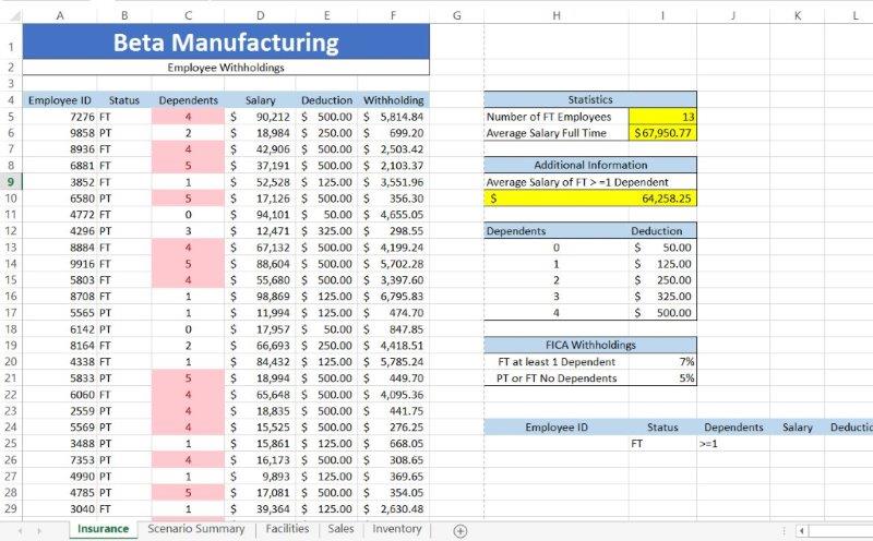
| 2 | Group all the worksheets in the workbook and fill the range A1:F1 from the Insurance worksheet across all worksheets maintaining the formatting. Ungroup the worksheets after the fill is complete and ensure the Insurance worksheet is active. | 4.000 |
| 3 | Click cell I5 and enter a function that determines the number of full-time employees, (FT). | 2.000 |
| 4 | Enter a function in cell I6 that determines the average salary of all full-time employees. Format the results in Accounting Number Format. | 2.000 |
| 5 | Enter a lookup function in cell E5 that returns the tax deduction amount for the number of dependents listed in the cell C5. Use the table in range H13:I17 to complete the function. The maximum deduction is $500.00; therefore, employees with more than four dependents will receive no additional deductions. |
2.000 |
| 6 | Use Auto Fill to copy the function down, completing column E. Be sure to use the appropriate cell referencing. Format the data in column E with the Accounting Number Format. | 4.000 |
| 7 | Enter a logical function in cell F5 that calculates employee FICA withholding. If the employee is full-time and has at least one dependent, then he or she pays 7% of the annual salary minus any deductions. All other employees pay 5% of the annual salary minus any deductions. Copy the function down through column F. Format the data in column F with Accounting Number Format. | 3.000 |
| 8 | Apply conditional formatting to the range C5:C34 that highlights any dependents that are greater than 3 with Light Red Fill and Dark Red Text. | 4.000 |
| 9 | Click cell H10, and enter an AVERAGEIFS function to determine the average salary of full-time employees with at least one dependent. Format the results in Accounting Number Format. | 3.000 |
| 10 | Use Advanced Filtering to restrict the data to only display full-time employees with at least one dependent. Place the results in cell A37. Use the criteria in the range H24:M25 to complete the function. | 2.000 |
| 11 | Ensure that the Facilities worksheet is active. Use Goal Seek to reduce the monthly payment in cell B6 to the optimal value of $6000. Complete this task by changing the Loan amount in cell E6. | 5.000 |
| 12 | Create the following three scenarios using Scenario Manager. The scenarios should change the cells B7, B8, and E6.
Good Most Likely Bad Create a Scenario Summary Report based on the value in cell B6. Format the new report appropriately. |
5.000 |
| 13 | Ensure that the Facilities worksheet is active. Enter a reference to the beginning loan balance in cell B12 and enter a reference to the payment amount in cell C12. | 4.000 |
| 14 | Enter a function in cell D12, based on the payment and loan details, that calculates the amount of interest paid on the first payment. Be sure to use the appropriate absolute, relative, or mixed cell references. | 3.000 |
| 15 | Enter a function in cell E12, based on the payment and loan details, that calculates the amount of principal paid on the first payment. Be sure to use the appropriate absolute, relative, or mixed cell references. | 3.000 |
| 16 | Enter a formula in cell F12 to calculate the remaining balance after the current payment. The remaining balance is calculated by subtracting the principal payment from the balance in column B. | 2.000 |
| 17 | Enter a function in cell G12, based on the payment and loan details, that calculates the amount of cumulative interest paid on the first payment. Be sure to use the appropriate absolute, relative, or mixed cell references. | 3.000 |
| 18 | Enter a function in cell H12, based on the payment and loan details, that calculates the amount of cumulative principal paid on the first payment. Be sure to use the appropriate absolute, relative, or mixed cell references. | 3.000 |
| 19 | Enter a reference to the remaining balance of payment 1 in cell B13. Use the fill handle to copy the functions created in the prior steps down to complete the amortization table. | 3.000 |
| 20 | Ensure the Sales worksheet is active. Enter a function in cell B8 to create a custom transaction number. The transaction number should be comprised of the item number listed in cell C8 combined with the quantity in cell D8 and the first initial of the payment type in cell E8. Use Auto Fill to copy the function down, completing the data in column B. | 7.000 |
| 21 | Enter a nested function in cell G8 that displays the word Flag if the Payment Type is Credit and the Amount is greater than or equal to $4000. Otherwise, the function will display a blank cell. Use Auto Fill to copy the function down, completing the data in column G. | 7.000 |
| 22 | Create a data validation list in cell D5 that displays Quantity, Payment Type, and Amount. | 5.000 |
| 23 | Type the Trans# 30038C in cell B5, and select Quantity from the validation list in cell D5. | 2.000 |
| 24 | Enter a nested lookup function in cell F5 that evaluates the Trans # in cell B5 as well as the Category in cell D5, and returns the results based on the data in the range A8:F32. | 3.000 |
| 25 | Create a PivotTable based on the range A7:G32. Place the PivotTable in cell I17 on the current worksheet. Place Payment Type in the Rows box and Amount in the Values box. Format the Amount with Accounting Number Format. | 5.000 |
| 26 | Insert a PivotChart using the Pie chart type based on the data. Place the upper-left corner of the chart inside cell I22. Format the Legend of the chart to appear at the bottom of the chart area. Format the Data Labels to appear on the Outside end of the chart.
Note, Mac users, select the range I18:J20, on the Insert tab, click Recommended Charts, and then click Pie. Format the legend, and apply the data labels as specified. |
4.000 |
| 27 | Insert a Slicer based on Date. Place the upper-left corner of the Slicer inside cell L8. | 3.000 |
| 28 | Ensure the Inventory worksheet is active. Import the Access database eApp_Cap2_Inventory.accdb into the worksheet starting in cell A3.
Note, Mac users, download and import the delimited Inventory.txt file into the worksheet starting in cell A3. |
5.000 |
| 29 | Create a footer with your name on the left, the sheet code in the center, and the file name on the right for each worksheet. | 2.000 |
| 30 | Save and close the file. Based on your instructor’s directions, submit eApp_Cap2_Manufacturing_LastFirst.xlsx. |
0.000 |
| Total Points | 100.000 |
Leave a Reply to Team Libraay Cancel reply
- File Format (Solution File): MS-Excel .xlsx
- Version: 2016
- File Format(Guide): .PDF
I was scared to use this at first, but this actually worked! It was in my e-mail. Such a relief, I had no clue what I was doing. Libraay saved my life!
Dear Kass,
We are glad that we could assist you. Please feel free to reach us with your computer science projects at info@libraay.com for the most student friendly quotes and A+ solutions.
Team Libraay.
hi i have a question does it show you step by step how to solve it or does it just give you the answer?
thank you
Dear Riya Yelda,
You shall see three options for purchase for the project. Please select “How-To-Solve Guide (with screenshots)” for step by step guide for the project. Write to us at info@libraay.com for any assistance.
Team Libraay
What file do I use to open when it I receive it in my email? I tried a zip file manager and it was blank?
Dear Jayson Gibbs,
You may use any Zip utility like WinZip, 7-Zip etc to extract the files. For any further assistance, please write to us at info@libraay.com
Team Libraay
I was a little skeptical at first, but this ended up being the best $5 I’ve spent on something school related! Some of the results ended up being different at the end, but the screen shots were easy to follow and I passed my assignment with a 96%. So I’ll take it! Thank you!
Dear Ellie,
We apologize for a rather reply. Your comment got missed by our team.
We are glad that we could assist you. You may choose to send across your new projects/assignments to us at info@libraay.com for student friendly quotes and great quality solutions within promised deadlines. Looking forward to work with you more.
Team Libraay
I already bought this, but I haven’t gotten any email with the files. How long do i have to wait to receive them?
The issue has been resolved now. Please check your Inbox for an e-mail from us.
Team Libraay
I bought this, but I haven’t got an email with the files yet. How long do I have to wait to receive them?
All Libraay downloads are E-Mailed to your registered ID immediately after successful purchase. Please check the Inbox/Spam/Junk folder of your E-Mail for an E-Mail from info@libraay.com. If you still don’t get it, please write to us at info@libraay.com.
I haven’t gotten the file sent to my email and i checked my junk folder as well. Help?
As this is your institute’s ID, our domain may be blocked. Please share your personal ID where we can E-Mail your file(s).
For any future purchases, please use only E-Mail IDs which are not under firewall surveillance.