Office 2016 MyITLab MS-Excel Grader EX16_XL_VOL1_GRADER_CAP_HW – Software Training Books 1.4
-----View all Office 2016 MyITLab Grader Digital Solution Download Files-----
-----View all Office 2016 MyITLab Grader Digital Solution Download Files-----
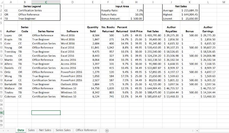
You are a vice president for a publisher of software training books. Your division publishes three series that focus on Microsoft Office and Windows. You want to analyze the sales data and calculate author royalties. You will format the worksheet, insert formulas and functions to perform calculations, sort and filter data to review specific book sales, and prepare a chart that compares sales by series.
Instructions:
For the purpose of grading the project you are required to perform the following tasks:
| Step | Instructions | Points Possible |
| 1 | Start Excel. Download and open the file named exploring_ecap_grader_h1.xlsx. | 0.000 |
| 2 | On the Data worksheet, select the range A6:K6, wrap the text, and apply Center alignment. Change the row height to 30 for row 6. | 3.000 |
| 3 | In cell F7 in the Data worksheet, insert a formula that calculates the percentage of books returned based on the number of books returned and the quantity sold. Copy the formula from cell F7 to the range F8:F22. | 4.000 |
| 4 | In cell H7 in the Data worksheet, insert a formula that calculates the net sales. This monetary amount reflects the number of books not returned and the unit price. Copy the formula from cell H7 to the range H8:H22. | 4.000 |
| 5 | In cell I7 in the Data worksheet, insert a formula that calculates the amount of the first author’s royalties. An author’s royalties are based on the Royalty Rate located in the Input Area and the respective Net Sales. Copy the formula from cell I7 to the range I8:I22. | 4.000 |
| 6 | In cell K7 in the Data worksheet, insert a formula that adds the first author’s royalty amount to the bonus. Copy the formula from cell K7 to the range K8:K22. | 4.000 |
| 7 | In cell J2 in the Data worksheet, insert a function to calculate the average net sales. In cell J3 insert a function to calculate the highest net sales. In cell J4 insert a function to calculate the lowest net sales. | 6.000 |
| 8 | Select the range L1:N2 in the Data worksheet, copy the selected data, and transpose the data when pasting it to cell A2. Delete the data in the range L1:N2. | 4.000 |
| 9 | Click cell C6 in the Data worksheet and insert a column. Type Series Name in cell C6. Click cell C7 in the Data worksheet and insert a lookup function that identifies the series code, compares it to the series legend, and then returns the name of the series. Copy the function you entered from cell C7 to the range C8:C22. Change the width of column C to 18. | 8.000 |
| 10 | Click cell K7 in the Data worksheet and replace the current contents with an IF function that compares the percent returned for the first book to the return rate in the Input Area. If the percent returned is less than the return rate, the result is $500. Otherwise, the author receives no bonus. The only value you may type directly in the function is 0 where needed. Copy the function you entered from cell K7 to the range K8:K22. | 5.000 |
| 11 | Select the range G7:G22 in the Data worksheet and apply the Percent Style format with one decimal place. Select the range K7:K22 and apply the Accounting Number Format. Merge and center the label Series Legend in the range A1:C1 in the Data worksheet. Apply Thick Outside Borders to the range A1:C4.
Note, the border type may be Thick Box Border, depending on the version of Office used. |
6.000 |
| 12 | Select Landscape orientation, adjust the scaling so that the data fits on one page, and set 0.1 left and right margins for the Data worksheet. | 4.000 |
| 13 | Click the Sales sheet tab, convert the data to a table, and apply Table Style Light 9. | 4.000 |
| 14 | Sort the data by Series Name in alphabetical order and then within Series Name, sort by Net Sales from largest to smallest. | 4.000 |
| 15 | Add a total row to display the sum of the Net Sales column. Change the column width to 14 for the Net Sales column. | 4.000 |
| 16 | Select the values in the Percent Returned column and apply conditional formatting to apply Light Red Fill with Dark Red Text for values that are greater than 9.9%. | 3.000 |
| 17 | Select the values in the Net Sales column and apply a filter to display only net sales that are less than $100,000. | 4.000 |
| 18 | Click the Net Sales sheet tab, select the range A3:D7, and create a clustered column chart. | 4.000 |
| 19 | Move the chart so that the top-left corner is positioned inside cell A9. Change the chart width to 4.66 inches and the chart height to 2.9 inches. | 3.000 |
| 20 | Link the chart title to cell A1. Format the value axis to display whole numbers only. | 2.000 |
| 21 | Format the chart title, value axis, category axis, and legend with Black, Text 1 font color. | 3.000 |
| 22 | Select the Series Sales tab, select the ranges A4:A7 and C4:C7 and create a pie chart. Move the pie chart to a chart sheet named Office Reference. Move the Office Reference chart sheet to the right of the Series Sales sheet. | 5.000 |
| 23 | Change the chart title to Office Reference Series. Apply bold and change the font size to 18 for the chart title. | 2.000 |
| 24 | Apply the Style 12 chart style and change the colors to Colorful Palette 4. | 4.000 |
| 25 | Display data labels in the Inside End position. Display Percentage data labels; remove the Value data labels. Apply bold, change the font size to 18, and then apply White, Background 1 font color to the data labels. | 6.000 |
| 26 | Ensure that the worksheets are correctly named and placed in the following order in the workbook: Data, Sales, Net Sales, Series Sales, Office Reference. Save the workbook. Close the workbook and then exit Excel. Submit the workbook as directed. | 0.000 |
Leave a Reply to Team Libraay Cancel reply
- File Format: MS-Excel .xlsx
- Version: 2016
What was the formula you put in for Series Name?
Dear Annika,
Please purchase the solution / tutorial guide to get the formulas.
where do i purchase solution / tutorial guide to get the formulas.
Please write to us at info@libraay.com for ordering the tutorial guide.
will the how to solve guide tell me how to do it step by step?
Yes, the tutorial guide contains step-by-step solution to guide you through solving the project; accompanied with screen shots.
Write to us at info@libraay.com for any further assistance.
Does the step by step show you how to do it in the video instead of using screenshots
Currently, No. Our tutorial guides are based on screen shots only for now.
Team Libraay
is there a video of how to do it instead of screenshots
Currently, No. Our tutorial guides are based on screen shots only for now.
Team Libraay
How long does it take to receive the file once the purchase has been made?
The file access links are E-Mailed immediately after successful payment. Please check your Inbox/Spam/Junk folders for an E-Mail from info@libraay.com. If you did not receive it, your domain would have stopped an E-Mail from us. You may write to us with an alternative E-Mail address and we can arrange the links.